The Climate Model GENIE
GENIE is a flexible framework for climate modelling that can be used to couple together different model components of varying complexity in order to provide an appropriate modelling tool for a wide range of possible applications. GENIE has modules that describe the ocean, the atmosphere, ocean biogeochemistry, marine sedimentary processes, weathering processes, terrestrial vegetation, sea-ice and ice-sheets.
The results presented on this
website derive from two different GENIE configurations, which we call GENIE-1
and GENIE-2. The principal difference between these two configurations is the
complexity of the atmospheric model.
GENIE-1
The GENIE-1 configuration applied
here couples together a low resolution intermediate complexity 3D ocean model
(GOLDSTEIN), a highly simplified 2D energy-moisture balance atmosphere (EMBM)
model, a simple model of sea-ice (which accounts for both thermodynamic and
dynamic effects) and a minimum spatial model of terrestrial vegetation (ENTS).
Although we include a vegetation module (as vegetation has a very significant effect on energy-moisture balance through, for instance, changes in albedo and
"surface roughness"), other modules which relate to the carbon cycle (such as
the ocean biogeochemistry module BIOGEM) are not included. These are not
relevant for the work described here as we are analysing the greenhouse gas concentration
profiles that are outputs of the Integrated Assessment Modelling.
The results presented on this
website are derived from emulators that have
been derived from a collection of 480 GENIE-1 simulations. Each of these
simulations produce plausible modern and glacial climates but have different input
values for 25 key physical parameters in order to quantify model uncertainty. For a more detailed description of the ensemble design see Holden et al. Climate Dynamics (2009). The ensemble has an
average climate sensitivity (equilibrium temperature change at doubled CO2) of 3.8ºC.
GENIE-1 is applied at an ocean
resolution of 36x36x8. It simulates ~3,000 years of "real-time" in 1 CPU hour.
GENIE-2
The GENIE-2 configuration applied
here also uses the ocean model GOLDSTEIN, but couples it to a 3D atmospheric
model (IGCM), a highly simplified sea-ice model and a simplified land surface
model (which does not model vegetation). The atmospheric model is substantially
more complicated than in GENIE-1 and contains the same dynamics as full GCMs,
albeit at lower resolution with a simplified representation of physical
processes such as clouds. The use of a 3D atmosphere enables more robust
estimates of changes at a regional level than is possible with GENIE-1, but is
a very much more demanding calculation - GENIE-2 is approximately 250x slower
than GENIE-1 in the configurations described here (GENIE-2 is itself orders of
magnitude slower than the most complex GCMs).
We also apply an ensemble
methodology to build emulators of GENIE-2, though this ensemble is at an earlier
stage of development than the GENIE-1 ensemble. The ensemble varies 19 key
atmospheric and ocean parameters to generate 122 plausible modern climate
states (with the single constraint that they are required to have a modern
global average temperature of between 9.5 and 19.5°C). The climate sensitivity
of this ensemble has not yet been calculated (10,000s CPU hours are require to
run the simulations to equilibrium) but has been estimated from the "Transient
Climate Response" to be 2.1°C. This is at the low end of the range of IPCC
climate sensitivity (2.1 to 4.4°C). In order to correct for this bias and
present a climate response that better reflects the consensus of IPCC models, we have scaled the spatial patterns generated with GENIE-2 to the global
average warming predicted by GENIE-1.
GENIE-2 is applied at a resolution of 64x32x8
(ocean) and T21 atmosphere with 7 vertical levels. It simulates ~12 years of
"real-time" in 1 CPU hour.
Uncertainty in climate models
The uncertainty associated with
climate predictions arises from three distinct sources:
1) "Forcing Uncertainty" (unknown
future greenhouse gas and aerosol emission scenarios, land use change etc)
which are the causes of climate change. This is by far the greatest source of
uncertainty associated with future climate change.
2) Model "Parametric Uncertainty".
Processes which occur on small spatial scales, such as the formation of clouds
or ocean eddies, cannot be modelled in detail but are instead represented by
parameterisations. These are relatively simple equations which are designed to
reproduce the large-scale averaged effect of these processes. The coefficients
(parameters) in these equations cannot always be derived from theory, and the
precise values are hence not known, although theoretical understanding or
empirical observations provides information on sensible parameter choices.
Within this range of possible input, the range of possible model output which
can arise is known as the parametric uncertainty.
3) Model "Structural Uncertainty".
This arises as a result of shortcomings of the model and is very difficult to
quantify as it is caused by process which are either not modelled or are poorly
understood, so that the consequences of their effects are (almost by
definition) not calculable.
The total Parametric and
Structural Uncertainty is known as "Model Uncertainty". The calculations
described in this website address all three of sources of uncertainty by
considering both model and forcing uncertainty.
The evaluation of model uncertainty in GENIE-1
Based
on: A
probabilistic calibration of climate sensitivity and terrestrial carbon change
in GENIE-1 Climate Dynamics, Holden
PB, Edwards NR, Oliver KIC, Lenton TM and Wilkinson RD.
This section describes a study to
quantify the uncertainty in "Climate Sensitivity" that arises from model uncertainty. Climate sensitivity is defined
as the equilibrium response to a doubling of atmospheric CO2.
Although the forcing is well defined, the climate response to this forcing is very
difficult to quantify precisely (and is the focus of much climate research) as
it results from a myriad of complex and interconnected physical, chemical and
biological feedback processes in the atmosphere, ocean, cryosphere and
biosphere.
An ensemble is a collection of
simulations which vary unknown model inputs in order to provide a
quantification of model uncertainty. Here we describe an ensemble of roughly
1,000 GENIE-1 simulations in each of three climate states.
1) Pre-industrial with forcing
similar to today, except atmospheric CO2 concentration is fixed at
1850 levels of 280ppm.
2) Last Glacial Maximum (LGM), Ice-age conditions with CO2 concentration of 190 parts per million and with large areas of the globe covered in ice.
3) CO2 concentrations
doubled from pre-industrial levels to 560ppm.
Each of the 1,000 simulations
applies a different set of values for 25 parameters. The ranges of these
parameters were deliberately chosen to be wide in an attempt to encompass parametric uncertainty as much as possible.
Furthermore, we do not require the model to accurately reproduce the modern
climate state. We only require it to reproduce the general characteristics of
the modern climate state (to illustrate, we require the presence of sea-ice off
the coast of Antarctica). This is in contrast to the more usual approach of
using a "tuned" model, whereby parameter values are chosen in order
to reproduce the climate state as closely as possible. Our approach is designed
to allow for model structural error. By accepting a wide range of both input
parameters and output states, we allow parametric uncertainty to dominate over structural uncertainty to produce a wide range of
model responses which cover the range of uncertain feedback strengths.
We then apply a statistical approach
known as "Bayesian calibration" to calculate probability weightings
for each of the 1,000 parameter sets, based on how well each simulation
reproduces observed LGM cooling. These probability weightings are then applied
to the calculation of the climate response to elevated atmospheric CO2,
providing a calibrated estimate for climate sensitivity and the associated
uncertainty.
The approach indicates that the climate
sensitivity is most likely to be 3.5ºC, with a 90% probability that it will lie
within the range 1.6 to 4.7ºC. This is similar to the range of IPCC estimates
of climate sensitivity of 2.1 to 4.4ºC, derived from 19 state of the art GCMs (with
an average of 3.2ºC).
We do not consider only climate
sensitivity, but also use the model to consider the possible responses of other
important aspects of the Earth System, such as changes in sea ice and ocean
circulation. In particular, we consider the response of vegetation to global
warming and estimate a 37% probability that under doubled CO2, the
terrestrial biosphere will stop absorbing CO2 but instead begin to
emit additional CO2 due to increased plant respiration rates in
a warmer world.
Emulation of GENIE-1 and GENIE-2
A tool that has been applied for
much of this work is emulation, whereby the output of the model is
fitted to relatively very simple (and very fast) functional forms. The power of
emulation is that it can be used to investigate large numbers of different
model set-ups (e.g parameterisations or forcing scenarios).
The emulation of the climate
models is performed by fitting output variables to polynomial functions of
input parameters. The building of the emulator proceeds by successively adding
terms in an attempt to best describe the model output. In order to avoid
over-fitting the data, a test known as the "Bayes Information Criteria" is
applied each time a new term is added. This test favours an improved fit to the
data, but penalises the addition of extra terms, and so attempts to find a
minimum adequate model which best fits the data while minimising the number of
terms in the emulator.
Emulation of GENIE-1
To emulate GENIE-1, we have built
12 emulators which describe 3 outputs of the model (change in surface
temperature, change in vegetative carbon, change in fractional vegetation
cover) averaged over 4 large land masses (North America, South America,
Northern Hemisphere Eurasia/Africa and Southern Hemisphere
Asia/Africa/Australasia).
Emulation of GENIE-2
To emulate GENIE-2, we have
developed an approach to emulate 2D spatial fields of change. We have applied
this to emulate fields of warming over the next century. The approach uses the
technique of "Empirical Orthogonal Functions" (EOF).
This technique breaks down a set of
fields (here the different fields that are produced across an ensemble of
simulations) into a set of 2D orthogonal fields which describe the principal
patterns of spatial variability across the ensemble. Their primary purpose is
to reduce the large number of variables that are required to describe a set of
spatial fields, whilst retaining a full description of the variability of the
spatial pattern.
Typically the first 5 EOFs are
sufficient to capture ~90% of simulated variability. The Principal Components (PCs) of each EOF define the sign
and magnitude associated with that EOF in order to reproduce any given
simulated field. i.e. once the EOFs have been derived, knowledge of only five
numbers (the PCs) is sufficient to construct a good approximation to the
simulated field.
Just as the simulated field is a
function of the model parameters, so are the PCs. As such, they can be emulated
as a function of the model parameters. These emulators can then be used to
construct an emulation of the field from any arbitrary choice of inputs.
Here we emulate the first 5 PCs as
cubic functions of the 19 physical parameters (which generate model
uncertainty) and 3 Chebyshev coefficients (that
describe the greenhouse gas concentration profiles). So in order to derive the
warming field and uncertainty associated with a given concentration profile we
perform the following steps
1) solve to find the Chebyshev coefficients which best describe the concentration profile
2) apply these coefficients to derive an emulated ensemble of PC values (we apply each of the 122 different model parameterisations to the emulator together with the Chebyshev coefficients to generate a range of PC values)
3) Derive 122 emulated fields of temperature changes by combining the emulated PCs with the EOFs
4) Calculate the mean and standard
deviation of these 122 fields which describe the emulated warming and the
uncertainty in the prediction.
5) Scale the emulated warming according to give
the same globally averaged warming as emulated by GENIE-1 for the same
concentration pathway. This is done to correct for the bias that results from
the fact that GENIE-2 has a climate sensitivity (~2.1ºC) which is at the lower
end of the range of IPCC models (2.1 to 4.4ºC). The GENIE-1 ensemble has a
climate sensitivity of 3.8ºC which is a better (though now slightly high)
representation of the range of IPCC models.
Historical and Future Forcing Uncertainty
The climate forcing is expressed
in terms of effective CO2. This is the equivalent amount of CO2 that would provide the same total forcing as the sum of all greenhouse gases
(we consider CO2, CH4 and N2O and ozone),
anthropogenic aerosols and, for historical forcing, solar variability, volcanic
eruptions and land-use change.
The concentration pathways for
effective CO2 are separated into two periods, historical (1850-2005)
and future (2005-2105).
Both ensembles of simulations
(GENIE-1 and GENIE-2) are "spun-up" to be in equilibrium at pre-industrial
concentrations of CO2 of 280ppm. From these spun-up states, the
simulations are allowed to change, firstly in response to historical emissions
and then in response to different possible future emissions. It is necessary to
include the historical forcing (1850-2005) as the present climate is not in
equilibrium with current levels of atmospheric CO2. This is
primarily because of the large "thermal inertia" of the ocean which means that the
ocean does not warm fast enough to keep pace with the rate of greenhouse gas
emissions.
Historical Forcing
The historical forcing is derived
from Nozawa et al (2005) which expresses the effects of each the above forcing
components as a "radiative forcing". These are converted into an equivalent
effective CO2 concentration (Radiative Forcing = 5.35 x ln (CO2e
/280ppm) Wm-2).
Future Forcing
The output of TIAM is converted
into an equivalent CO2 concentration profile. This profile can take
any arbitrary path to reach any arbitrary level of CO2e in 2105.
To convert this arbitrary profile
into a simple analytical form (which can be emulated) we approximate it by the
first three "Chebyshev polynomials" according to the equation
Ce = C0 +
0.5 * (A1 (t +1) + A2 (2t2 -2) + A3 (4t3 - 4t))
where Co is the effective CO2 concentration in 2005 (=393 ppm), t is time and A1, A2 and
A3 are the three coefficients, technically these are linear combinations of the first three classical Chebyshev coefficients. For completeness, it is
worth noting that time is mapped onto the range (-1, 1) with -1 being 2005 and
1 being 2105 so that the value of A1 is equal to the total change in
CO2e between 2005 and 2105.
To build the ensembles and emulators
of GENIE-1 and GENIE-2 we produce emissions scenarios by allowing these three
coefficients to vary over ranges that cover likely future emissions scenarios.
To investigate the consequences of
an emissions scenario produced by TIAM, we solve for the three coefficients that
best describe this pathway. These three coefficients then provide the necessary
input for the GENIE emulators to calculate an estimate for the climate change
(and associated uncertainty) that would arise from this TIAM scenario.