SynsCOP15 - Technology/energy model

Technology / Energy Model

TIAM (for TIMES Integrated Assessment Model)

The TIMES Integrated Assessment Model (TIAM) is a detailed, technology-rich global model based on the TIMES paradigm. It is the outcome of global modeling work over the past decade by researchers of KanLo. The model has been actively promoted and partly funded by ETSAP over the past few years.

It is a multi-region partial equilibrium model of the energy systems of the entire World divided in several regions. The regional modules are linked by trade variables of the main energy forms (coal, oil, gas) and of emission permits. Thus, impacts on trade (terms of trade) of environmental policies are taken into account. TIAM's planning horizon extends from 2000 to 2100, divided into periods of varying lengths, suitably chosen.

TIAM is a global instance of the TIMES model generator (full documentation and applications in www.etsap.org/documentation.asp), where a bottom-up, detailed technological representation of each economic sector is combined with key linkages to the macroeconomy. TIMES has evolved from its MARKAL forebear and has benefited from many improvements sponsored by ETSAP over the last 8 years.

The TIAM incarnation of TIMES is described in Loulou (2007) and in Loulou and Labriet (2007).

Regions

The version of TIAM used for this application includes 16 regions: Africa, Australia, Canada, Central and South America, Central Asia and Caucase, China, Europe (EU27+), India, Japan, Middle-East, Mexico, Other Developing Asia, Other Eastern Europe, Russian Federation, South Korea, USA.

Economic Rationale

The model is driven by a set of 42 demands for energy services in all sectors: Agriculture, Residential, Commercial, Industry, (for and Transportation services. Examples of energy services are: lighting, water heating, space cooling, etc. (residential and commercial sectors), tons of aluminium, of iron&steel, etc. to produce (industry), vehicle-km to drive by cars, by bus, etc. (transport). Demands for energy services are exogenously specified only for the Reference scenario, and have each a user-defined own-price elasticity. Therefore, each demand may endogenously vary in alternate scenarios, in response to endogenous price changes. Although TIMES does not encompass all macroeconomic variables beyond the energy sector, accounting for price elasticity of demands captures a major element of feedback effects between the energy system and the economy. The model thus computes a partial equilibrium on world-wide energy and emissions markets that maximizes the discounted present value of global surplus, representing the surplus of all consumers and producers (practically, the LP minimizes the negative of the surplus, which is then called the system cost). As described in its general form by Takayama and Judge (1971) and, in the case of Bottom-Up energy models, in Loulou and Lavigne (1996), the computation of the supply-demand partial equilibrium is equivalent to the maximization of the total surplus, which is a concave maximization problem. In TIAM, all nonlinear expressions possess the required concavity or convexity property, and all are approximated by piece-wise linear expressions before treatment via Linear Programming.

The cost portion of the surplus objective is constructed as follows: first, each period's investment and dismantling costs are annualized, using hurdle rates that are sector dependent. These annualized investment costs are then added to annual costs (fixed and variables), to form the total annual costs. The stream of annual costs is then discounted to year 2005 using the general discount rate of 5% (the interest rate). All costs are expressed in USD2005. Hurdle rates are important in influencing the competition between technologies in each subsector (a large hurdle rate favors technologies with small investment expenditures). The hurdle rates range from 6% to 9% per year for large utilities and heavy industries, to more than 25% per year for investments in the residential, commercial, and private transportation sectors. The hurdle rates were obtained from the work done in the European Union integrated project NEEDS (Cosmi et al, 2006). A salvage value term is subtracted from the cost objective in order to account for the residual value of technologies still extant after the end of the horizon, and thus attenuate the end-of-horizon bias. TIAM, as all TIMES models, tracks all financial flows in much detail in order to account for the time lags and lead-times existing between the investment decisions, the actual commissioning, decommissioning, and dismantling of technologies.

Technological dimension of TIAM

The model's variables include the investments, capacities, activity levels of all technologies at each period of time, plus the amounts of energy, material, and emission flows in and out of each technology. Trade links are also represented as technologies between two regions, with their own costs and efficiencies; such endogenous trade of crude oil, petroleum products, gas, liquefied natural gas, coal, as well as greenhouse gas permits, if wanted, is included in TIAM.

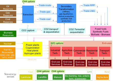
TIAM contains explicit descriptions of more than one thousand technologies and one hundred commodities (energy forms, materials, emissions) in each region, logically interrelated in a Reference Energy System (Figure 1). Each technology has its own technical and economic parameters. Such technological detail allows precise tracking of capital turnover, and provides a precise description of technological competition. The model's scope covers extraction, processing, conversion, trading, and end-uses of all energy forms. Primary resources are disaggregated by type (e.g. proven vs. future natural gas reserves, connected vs. not, frontier gas, CBM, associated gas, etc). Each type of non renewable resource is described in each region by means of a step-wise supply curve (3 steps) for the cumulative amounts in the ground, technical annual extraction limits, and fixed and variable costs, thus constituting a compound step-wise supply curve for each primary energy form (coal, oil, gas). All renewable energy forms have annual potentials in each region, also with multiple steps.

The TIMES model generator contains more than 30 types of standard constraints, ranging from flow balance equations to capacity transfer equations, to bounds on the utilization rate of technologies, to technical equations that simulate the utilization regime of some electricity generation plants, etc. In addition, there are a number of user-defined constraints that express specific regional, sectoral, and technological conditions. For example, in many cases, the penetration of new technologies or of new fuels is partially controlled by upper bounds that are progressively relaxed as time goes on. In some end-use sectors, there are also fuel share constraints that impose certain bounds on the market shares of some fuels (e.g. natural gas use is often unavailable in parts of non urban residences, and thus can never conquer the entire end-use sector). These additional constraints confer additional realism to the technological competition.

The reference energy system of TIAM

Emissions

TIAM explicitly models emissions of CO2, N2O and CH4 from all anthropic sources (energy, industrial processes, land, agriculture, waste) directly related to energy consumption but also to processes themselves (eg. N2O from nitric and adipic acid industry; CH4 from landfills, etc.).

The CO₂, CH₄ and N₂O emissions related to the energy sector are explicitly represented by the energy technologies included in the model. Each technology includes the appropriate emission coefficients. In addition, there are measures to destroy N2O, others to burn methane (by flaring or electric power plants), and still others to capture CO2 and store in underground or undersea in a variety of reservoirs (deep saline aquifers, exhausted wells, enhanced oil recovery, coal seams, ocean). Capture and geological storage of CO2 is available at electric power plants, at oil wells, at plants that produce synthetic fuels, and at hydrogen plants. In each case, the capture is not complete (around 9-11% of the CO2 escapes to the atmosphere). Finally, atmospheric CO₂ may be partly absorbed and fixed by biological sinks such as forests; the model has six options for forestation and avoided deforestation, as described in Sathaye et al. (2005) and adopted by the Energy Modelling Forum, EMF-21 and 22 groups.

CO₂, CH₄ and N₂O emissions from non energy sectors are also included in order to correctly represent the radiative forcing induced by them. These emissions are:

- CH₄ from landfills, manure, rice paddies, enteric fermentation, wastewater, based on the EMF-22 data;

- N₂O from agriculture, based on the EMF-22 data;

- CO₂ from land-use, based on the Reference scenario of the United States Climate Change Science Program (MIT) presented in Prinn et al. (2008), which shows a quasi linear decline from 2.7 GtCO2 in 2010 to 0.1 GtCO2 in 2100.

Regarding non-energy N2O and CH4, only about 40-45% of the emissions from landfills and manure can be destroyed or burned. Mitigations options of until 20% of CH4 and N2O emissions from agriculture activities are also included, at a cost of 75 to 250$/tCO2eq, representing the implementation of advanced agriculture practices.

Emissions from some Kyoto gases (CFC's, HFC's, SF6) are not explicitly modeled, but a special forcing term is added as described in the next paragraph. Emissions of chemically active gases such as NOx, CO, VOC's are not modeled either. Their influence on the life cycles of GHG gases is implicitly accounted for in the concentration equations for the three main GHG's (IPCC AR4, 2007, vol.1, ch. 2), but only through the calibration phase of the equations (Nordhaus and Boyer, 1999).

Climate Module

The climate module is directly inspired by the Nordhaus-Boyer (1999) model, but underwent several changes in order to (i) represent the three gases separately, (ii) use more precise forcing expressions based on the non controversial equations provided by the IPCC (2001, WG1), (iii) be linearized, and (iv) accommodate the variable-length periods of TIAM. The module allows the user to simulate climate targets either in terms of concentrations, of forcing, or of temperature change.

The climate module also uses the most recent information provided by the IPCC, such as the Global Warming Potentials (298 for N2O and 25 for CH4) and the radiative forcing sensitivity to atmospheric CO₂concentration doubling (3.7 W/m²).

The climate model proposed by Nordhaus and Boyer and used in TIAM has been compared to more sophisticated climate models and found quite accurate within the range of emissions usually considered (Nordhaus and Boyer, 1999).

It consists of three sets of equations, detailed below.

- The first set accepts as inputs the emissions of three Greenhouse gases, CO2, CH4, and N2O, from all sources (energy, industrial, land-use), net of geological capture and storage or destruction, and calculates the atmospheric concentrations of the three gases using recursive dynamic equations. The CO2 life cycle includes three layers (atmosphere, upper ocean, deep ocean, Nordhaus and Boyer, 1999). The CH4 and N2O atmospheric concentrations are each governed by a one-box exponential decay model, as used for example in Monni et al. (2003) and Manne and Richels (2004).

- The second set of equations accepts as inputs the atmospheric concentrations and calculates the atmospheric radiative forcings of these three gases via their three specific functional forms (IPCC AR4, 2007, vol. 1, ch. 2). The total forcing is then computed by adding up these three forcings plus a fourth (exogenous) forcing due to Kyoto GHG's that are not explicitly modeled in TIAM, so as to account for the totality of the Kyoto gases. The exogenous forcing trajectory was established from the values indicated in the AR4 (IPCC 2007, vol 1, ch 2) and extended to 2100 using the assumptions from Prinn et al (2008). The forcing expressions for the three gases CO2, CH4 and N2O are non linear and non convex, but have been linearized in the TIAM module. The linear approximation was tested within the range of interest of concentrations (i.e. from 400 to 700 ppmv CO2-equivalent). The maximum error thus incurred is less than 3%, which is well within the range of uncertainty attached to climate equations. The approximations are used only to compute the constraints on forcing, but the exact expressions are used when reporting the results. Note that the reference case emissions do exceed the 700 ppmv level, but this is of no consequence, as this scenario does not involve upper bounding.

- The third set of equations accepts as inputs the total radiative forcing and recursively calculates the yearly change in mean global temperature in two layers. The first layer consists of the atmosphere and the ocean surface, the second layer is the deep ocean. Heat transfer equations between these layers are represented in the equations. The transition from forcing to temperature change involves a crucial parameter, the climate sensitivity C_s, which is subject to much uncertainty. In section 3.3, we indicate how this uncertainty is explicitly taken into account in this research.

Some references

Other References

Cosmi, C., Blesl, M., Kanudia, A., Kypreos, S., Loulou, R., Smekens, K., Salvia, M., Van Regemorter, D., Cuomo, V., 2006. Integration of country energy system models in a Pan European framework for supporting EU policies. In: Brebbia, C.A. (Ed.), Environmental Economics 2006. In: WIT Transactions on Ecology and the Environment, vol. 95. WIT Press Southampton, UK, pp. 97-106. ISSN 1743-3541.

Loulou, R., D. Lavigne, 1996, "MARKAL Model with Elastic Demands: Application to GHG Emission Control", in Operations Research and Environmental Engineering, C. Carraro and A. Haurie eds., Kluwer Academic Publishers, Dordrecht, Boston, London, 1996, pp. 201-220.

Takayama, T., G. G. Judge, 1971, Spatial and Temporal Price and Allocation Models, North Holland, Amsterdam, 1971.

IPCC , 2007, Climate Change 2007: The Physical Science Basis. Contribution of Working Group I to the Fourth Assessment Report of the Intergovernmental Panel on Climate Change [Solomon, S., D. Qin, M. Manning, Z. Chen, M. Marquis, K.B. Averyt, M. Tignor and H.L. Miller (eds.)]. Cambridge University Press, Cambridge, United Kingdom and New York, NY, USA, 996 pp.

IPCC, 2001, Climate Change 2001: The Scientific Basis. Contribution of Working Group I to the Third Assessment Report of the Intergovernmental Panel on Climate Change [Houghton, J.T.,Y. Ding, D.J. Griggs, M. Noguer, P.J. van der Linden, X. Dai, K. Maskell, and C.A. Johnson (eds.)]. Cambridge University Press, Cambridge, United Kingdom and New York, NY, USA, 881 pp.

Manne, A., Richels R., 2004: MERGE: A Model for Evaluating the Regional and Global Effects of GHG Reduction Policies. http://www.stanford.edu/group/MERGE/

Monni, S., Korhonen, R. & Savolainen, I. 2003. Radiative Forcing Due to Anthropogenic Greenhouse Gas Emissions from Finland: Methods for Estimating Forcing of a Country or an Activity. Environmental Management, vol 31, No. 3, p. 401-411.

Nordhaus W. D. and J. Boyer, 1999, Roll the DICE Again: Economic Models of Global Warming, Yale University, manuscript edition.

Prinn, Ronald, Sergey Paltsev, Andrei Sokolov, Marcus Sarofim, John Reilly, and Henry Jacoby, 2008, "The Influence on Climate Change of Differing Scenarios for Future Development Analyzed Using the MIT Integrated Global System Model", MIT Joint Program on the Science and Policy of Global Change, Report No. 163, September 2008

Sathaye J., Makundi W., Dale L., Chan P., and Andrasko K. (2005). Estimating Global Forestry GHG Mitigation Potential and Costs: A Dynamic Partial Equilibrium Approach. LBNL - 55743.

Documentation on TIAM

general documentation and more detailed climate module description :

http://www.kanors.com/DCM/Tiam/Docs/Index.aspx

Result analysis :

http://www.kanors.com/DCM/Tiam

Documentation on TIMES model

http://www.etsap.org/documentation.asp